Credit strategies normally establish return and risk parameters. A credit strategy is typically designed to achieve a constrained objective.
VOCAB:
Spread Duration – measures the effect of a change in spread on a bond’s price. SD provides the approximate percentage increase
Average OAS – A portfolio’s credit quality can also be estimated using OAS. To calculate a portfolio’s average OAS, each bond’s individual OAS is weighted by its market value. It does not fully account for the risk of credit spread volatility.
Average Spread Duration – Similar to average OAS, however, a weighted-average spread duration can account for the risk of credit spread volatility.
Duration times spread (DTS) – A measure of credit quality that attempts to account for both average OAS and average spread duration. DTS is Bond Duration * OAS. It is sometimes useful to calculate Duration using DTS/OAS.
There are two important credit strategy approaches: a bottom up approach and a top down approach.
Bottom Up Approach
The bottom-up approach to credit strategy is sometimes called a “security selection” strategy. The key feature of the bottom-up approach is the assessment of the relative value of individual issuers or bonds. This approach is most appropriate for analyzing companies that have comparable credit risk, as opposed to those companies whose credit risk varies considerably (for example, investment-grade and high-yield companies).
The bottom-up manager would start with identifying the universe of bonds to consider, then divide that universe into sectors such as auto-related and mortgage-backed securities (MBS). Typically the manager is being measured against a benchmark and would match benchmark weights but over- or underweight individual securities or issuers. The manager should determine if the sector divisions in the benchmark are reasonable. For example, the manager may believe MBS is too broad a sector and differentiating government versus privately backed MBS will reveal important differences in risk or expected return.
The manager then looks for relative misvaluation within each sector to determine individual securities to select. The evaluation must weigh compensation (expected excess return) versus credit risks (credit spread, credit migration, default, and liquidity risks).
Gathering information to assess the credit risks is critical. This can include historical default rates (p) and loss rates (L) as well as charting past spread relationships. For example, a particular auto company’s bonds trade at spreads that are wider than the issuer’s average and wider than other auto companies. As long as the analyst is convinced there are no unaccounted for risk differences, overweight that company’s bonds.
The previous excess return model can be used in this analysis:
XR = (s × t) − (Δs × SD) − (t × p × L).
Assuming the analyst does not expect spreads to change, this issue becomes comparing the incremental spread earned versus estimated default losses. This is complicated because the factors are interrelated; bonds with higher expected default losses (a negative) usually have higher spread (a positive). Typically, the manager will select the bonds with highest XR but there are exceptions to this. The portfolio may already be overweighted in that issuer and need to diversify into less attractive XR bonds. The manager may also need to select bonds with lower XR to emphasize high liquidity or to meet an overall portfolio duration constraint.
Spread curves are another useful bottom-up tool. Spread Curve for Two Companies provides an example of how to use such curves.
Spread Curve for Two Companies
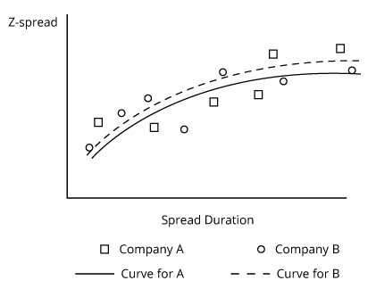
Based on Spread Curve for Two Companies:
- In general, bonds of company B offer slightly higher spread. Assuming the two issuers are equal in all other regards, the B bonds offer better excess return and are more attractive.
- Both issuers have several available issues. Any specific bond issue that plots above (or below) the issuer’s curve is potentially more attractive (or unattractive) for purchase.
- These are tentative conclusions and the bonds should be examined carefully for other considerations such as differences in:
- Liquidity.
- Date of issuance; older issues are generally less liquid.
- Pending new supply; if the issuer is about to issue a new security of similar remaining maturity the older issue is likely to decline in liquidity.
- Seniority in bankruptcy; subordinated debt is likely to experience greater loss (less recovery) in bankruptcy.
- Size of issue and total issuance outstanding by issuer; generally larger individual issues and total issuance make it economical for more investors to analyze and follow the bonds. Therefore, the increased issuance is often associated with better liquidity and higher bond prices. However, there can be too much supply of a given issue and issuer, leading to the opposite effect. The supply may saturate the market demand, leading to less liquidity, wider bid-ask, and higher credit spreads. Excessive issuance could also be associated with too much leverage and declining credit quality.
Final credit portfolio construction involves identifying the optimal risk exposures and best relative value holdings, and is likely to involve compromise.
- In specifying exposure to credit risk, the manager should consider both spread duration and market value allocation.
- Spread duration measures expected percent change in value from spread change. .
- In contrast, for HY and bonds where default risk is high, market value allocation is the more relevant measure of credit risk.
- The manager must also be prepared to compromise in selecting best relative value. The first, second, or even third choice bond may turn out to be unavailable for purchase. The manager can:
- Move down his relative value list and find the best available substitute bond.
- Temporarily invest in a suitable index fund (or use swaps or other derivatives to replicate such exposure) until the desired bonds are available.
- Temporarily hold cash and not have the desired bond market exposure until the desired bonds are available.
Top Down Approach
The top-down approach focuses on macro factors that are likely to affect the credit portfolio. Relevant factors include strength of economic growth and corporate profits. Stronger growth and profits are associated with decreasing spread and suggest moving down in credit quality for greater relative price gains. Top-down managers may use this relationship to identify when to focus on HY versus IG.
Top-down can also be used to identify sectors of the market most likely to improve (or deteriorate) and the manager can overweight (or underweight) those sectors. This analysis could also be used by the bottom-up manager to identify sectors for more targeted individual security analysis.
Top-down may focus on historical patterns such as the credit cycle and credit spread change. The credit cycle refers to variations in real economic growth and default rates. The two are negatively correlated in general, though it is not a perfect relationship.
The default rate and spreads are also highly correlated so the manager must generally be able to anticipate the next change in economic conditions to add value. For example suppose real growth is very low, defaults are high, and OAS for HY bonds is well above average; there is no particular opportunity because the high spread is compensation for high default losses. But if the manager has insight that the economy and growth rate are going to improve, it is an opportune time to move into HY.
The top-down manager would likely vary the portfolio’s average credit rating upward to a higher (or downward to a lower) rating in anticipation of weaker (or stronger) than consensus expectations for economic growth. The manager should consider how the portfolio’s average quality is calculated. Often, a numeric sequence is assigned to each rating (e.g., AAA = 1, AA+ = 2, AA = 3, AA– = 4). The portfolio’s market value weighted average rating is then calculated. This approach can understate exposure to credit risk because default rates and losses tend to increase rapidly as the rating declines. Other more complex “non-arithmetic” scales assign a number that increases much more rapidly than 1, 2, 3, 4 as credit rating declines (e.g., 1, 10, 20, 40 is used by Moody’s). Non-arithmetic portfolio averages will show that exposure to credit risk increases at a faster than linear rate, as bond rating declines.
Portfolio average OAS (or other spread) and spread duration are also calculated based on market value weighted average. A higher spread indicates the portfolio has greater exposure to credit risky assets. But spread duration indicates how much the portfolio will change in value if spread changes. Combining the two as duration times spread (DTS) provides a more comprehensive indication of credit risk than either alone.
The credit portfolio manager can also use historical spread between credit risky sectors to assess relative attractiveness.
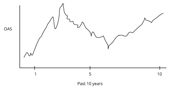
- Suppose a manager examines OAS for High-Yield Sector, believes the first 5 years of data are distorted by a major financial crisis, the last 5 years are relevant, and spread is mean reverting; that manager would find HY attractive because the spread differential is visually greater than the average of the last 5 years.
- Suppose another manager believes future economic conditions for the next few years will be much worse than consensus expectations; that manager would likely favor IG because the current spread reflects consensus views and economic deterioration should lead to spread widening. Spread widening is a more serious risk in HY than in IG.
Plotting the historical spread for other relationships is also useful. A manager could track the spread difference between 15- and 5-year A-rated bonds to gain perspective on the past relationship and as a starting point for developing a view on how the spread may change. If the manager sees the pick-up in yield for buying 15-year rather than 5-year bonds is average, but the manager forecasts a large increase in 15-year bond issuance, she may expect the spread to increase and overweight the 5-year sector now.
OAS for High-Yield Sector