
Taxes on investment returns have a substantial impact on performance and future accumulations.
Models enable the investment adviser to evaluate potential investments for taxable investors by comparing returns and wealth accumulations for different types of investments subject to different tax rates and methods of taxation.
Simple Tax Environments
One of the most straightforward methods to tax investment returns is to tax an investment’s annual return at a single tax rate, regardless of its form. Accrual taxes are levied and paid on a periodic basis, usually annually, as opposed to deferred taxes that are postponed until some future date.
FVIFAT = [1 + r(1 − ti)]n
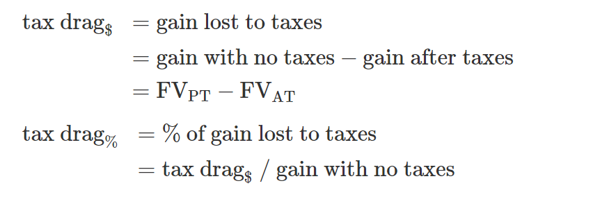
For accrual taxation r(1 − ti) is the after-tax rate of return so the computation is simply the after-tax value of a single initial currency unit invested. However, the ultimate effect of taxes on future value is complicated. One way to measure the effect is tax drag. Tax drag can be computed as both an amount and as a percentage. For example, for a U.S. investor:
Capital gains taxes are applied only to the gain in value on an asset. Generally, the timing of the tax can be controlled as it is only imposed when the asset is sold. By deferring the tax, the benefits of pretax compounding of return can be realized to lower the tax drag. If the initial starting value for the analysis period is the tax cost basis of the investment (i.e., the basis, B, equals 1.00), the future value of an investment after-tax under capital gains taxation is:
- FVIFAT = (1 + r)n(1 − tcg) + tcg
The advantage of the formula is it can be adjusted for the tax implications of a basis other than 1.00 and the resulting additional tax issues. It becomes:
- FVIFAT = (1 + r)n(1 − tcg) + tcgB
B = cost basis / asset value at start of period n
For capital gains taxes, it can be generalized that:
- Unlike accrual taxation, there is no lost compounding of return due to paying taxes periodically. All tax is paid at the end of the time horizon.
- The tax drag amount will increase as the time horizon and/or rate of return increase because the tax will be on a larger pretax ending value.
- The relationship of the tax drag percentage and stated tax rate will depend on the basis (B):
- If there is no initial unrealized gain or loss and B equals 1.00, the tax drag percentage is equal to the tax rate.
- If there is an initial unrealized gain and B is less than 1.00, the tax drag percentage is greater than the tax rate because there is an additional initial gain subject to tax.
- If there is an initial unrealized loss and B is greater than 1.00, the tax drag percentage is less than the tax rate because the portion of the return earned during the period back to the cost basis is untaxed.
In taxation, cost basis is generally the amount that was paid to acquire an asset. It serves as the foundation for calculating a capital gain, which equals the selling price less the cost basis. The taxable gain increases as the basis decreases. In consequence, capital gain taxes increase as the basis decreases.
If the cost basis is expressed as a proportion, B, of the current market value of the investment, then the future after-tax accumulation can be expressed by simply subtracting this additional tax liability from the capital gains equation:
- FVIFcgb = (1 + r)n(1 – tcg) + tcg – (1 – B)tcg
Notice that if cost basis is equal to the current market value of the investment, then B = 1 and the last term simply reduces to the capital gains equation. The lower the cost basis, however, the greater the embedded tax liability and the lower the future accumulation. Distributing and canceling terms produces
- FVIFcgb = (1 + r)n(1 – tcg) + tcgB
A wealth tax is imposed on total value, not just on return.
The future value of an investment after-tax under wealth taxation is:
- FVIFAT = [(1 + r)(1 − tw)]n
Compared to the accrual tax formula (FVIFAT = [1 + r(1 − ti)]n), the tax applies to end of period value (1 + r) and not just to return (r) each period. For the same tax rate, the effect of a wealth tax is much larger than for the other forms of taxation because the wealth tax applies to both start of period value and return earned. As a result, wealth tax rates tend to be lower than accrual or capital gains tax rates.
Blended Taxing Environments
Portfolios are subject to a variety of different taxes depending on the types of securities they hold, how frequently they are traded, and the direction of returns.
The different taxing schemes mentioned above can be integrated into a single framework in which a portion of a portfolio’s investment return is received in the form of dividends (pd) and taxed at a rate of td; another portion is received in the form of interest income (pi) and taxed as such at a rate of ti; and another portion is taxed as realized capital gain (pcg) at tcg.
The remainder of an investment’s return is unrealized capital gain, the tax on which is deferred until ultimately recognized at the end of the investment horizon. These return proportions can be computed by simply dividing each income component by the total dollar return.
In this setting, the annual return after realized taxes can be expressed as
- r* = r(1 – piti – pdtd – pcgtcg)
In this case, r represents the pre-tax overall return on the portfolio.
A portion of the investment return has avoided annual taxation, and tax on that portion would then be deferred until the end of the investment horizon. Holding the tax rate on capital gains constant, the impact of deferred capital gain taxes will be diminished as more of the return is taxed annually in some way as described above. Conversely, as less of the return is taxed annually, more of the return will be subject to deferred capital gains. One can express the impact of deferred capital gain taxes using an effective capital gain tax rate that adjusts the capital gains tax rate tcg to reflect previously taxed dividends, income, or realized capital gains. The effective capital gains tax rate can be expressed as:
- T* = tcg(1 – pi – pd – pcg)/(1 – piti – pdtd – pcgtcg)
The adjustment to the capital gains tax rate takes account of the fact that some of the investment return had previously been taxed as interest income, dividends, or realized capital gain before the end of the investment horizon and will not be taxed again as a capital gain.
The future after-tax accumulation for each unit of currency in a taxable portfolio can then be represented by
- FVIFTaxable = (1 + r*)n(1 – T*) + T* – (1 – B)tcg
Although this formulation appears unwieldy, (1 + r*)n(1 − T*) + T* is analogous to the after-tax accumulation for an investment taxed entirely as a deferred capital gain. The only difference is that r* is substituted for r, and T* is substituted for tcg in most places.
Different assets and asset classes generate different amounts of return as interest income, dividends, or capital gain, and will thus have different values for pi, pd, and pcg.
Most accounts conform to none of these extremes, but can be accommodated by simply specifying the proper distribution rates for interest income, dividends, and capital gain. It is useful then to have an understanding of how investment style affects the tax-related parameters (e.g., pi, pd, and pcg).