Approaches to Return Attribution

Arithmetic Attribution and Geometric Attribution

Return attribution lets us identify which investment decisions taken by the fund manager were successful or unsuccessful in generating alpha. Return attribution also introduces precision into the feedback loop between the portfolio manager and their clients.

Return attribution is a technique that can both identify and quantify the performance of an actively managed fund versus its benchmark.

Arithmetic attribution is designed to explain any excess return—the differential between the return earned by the portfolio (R) and that of its appropriate benchmark (B).

Geometric attribution improves upon the arithmetic approach by classifying the geometric excess return (G).

• G = (1 + R) / (1 + B) − 1 = (R − B) / (1 + B)

In the derivation (for a given period), the geometric excess return (G) is equal to the ratio of the arithmetic excess return (R − B) over the wealth ratio of the portfolio’s appropriate benchmark (1 + B).

No smoothing approaches are needed to adjust the geometric attribution for effects over multiple time periods. However, with arithmetic attribution, adjustments are needed to smooth the subperiod effects over longer time periods.

In short, arithmetic attribution is best suited for use with nontechnical clients and in marketing reports, whereas geometric attribution is best suited for use with industry professionals.

Equity Return Attribution—The Brinson Model

The history of return attribution traces its roots from two key papers, Brinson and Fachler (1985) and Brinson, Hood, and Beebower (1986).

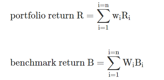
It is assumed that the total returns of the portfolio and benchmark are computed by adding up the multiplicative of the sector weights and returns. The following equations illustrate the computations and a simple calculation using the Brinson, Hood, Beebower (BHB) model:

where:

w_i = portfolio weight of the ith sector

R_i = portfolio return in the ith sector

W_i = benchmark weight of the ith sector

B_i = benchmark return in the ith sector

n = number of sectors

The BHB model approach quantifies the portfolio returns into three attribution effects: the allocation effect, the security selection effect, and the interaction effect.

The allocation effect refers to the portfolio manager’s decision to overweight or underweight specific sector weightings in the portfolio versus the portfolio benchmark. The allocation effect will quantify whether the portfolio manager’s decision to underweight the financial sector increased returns or lost value for the portfolio.

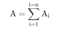
For a given sector, the contribution to allocation (A_i) is calculated as the difference between the portfolio and benchmark weights multiplied by the sector return for the benchmark.

• A_i = (w_i − W_i)B_i

The total portfolio allocation effect is simply calculated by adding up all of the contributions to allocation.

The next attribution effect in the Brinson model focuses on security selection —the value the portfolio manager either added or detracted from the portfolio by selecting individual securities within the sector and weighting the portfolio differently compared to the benchmark’s weightings.

For a given sector, the contribution to selection (Si) is calculated as the benchmark weight multiplied by the difference between the portfolio and benchmark sector returns.

• S_i = W_i(R_i − B_i)

The third component in the Brinson model is the interaction effect. It can be thought of as a residual amount that ensures the arithmetic return minus the relative benchmark is fully accounted for in the attribution analysis.

For a given sector, the contribution to interaction (Ii) is calculated as the difference between the portfolio and benchmark weights multiplied by the difference between the portfolio and benchmark sector returns.

• I_i = (w_i − W_i)(R_i − B_i)

Equity Return Attribution—Factor-Based Return Attribution

A frequently used attribution model is the fundamental factor model, where a portfolio’s sensitivity to additional factors can be tested.

The Carhart model calculates the excess return from active portfolio management investment decisions by determining the impact on the portfolio due to the following factors: (1) market index (RMRF), (2) market capitalization (SMB), (3) book value to price (HML), and (4) momentum (WML).

For more in-depth analysis, the Carhart model allows practitioners to remove the effects of known market factors to quantify the excess returns from active management decisions that are not accounted for in the Carhart model.

• R_p − R_f = a_p + b_p1RMRF + b_p2SMB + b_p3HML + b_p4WML + E_p

where:

R_p = portfolio return

R_f = risk-free rate

a_p = alpha or return above the expected return for the portfolio’s level of systematic risk

b_p = various portfolio factor sensitivities

RMRF = return on a value-weighted equity index above that of the one-month T-bill rate

SMB = small minus big, a size (market-capitalization) factor; equal to the difference between the average return on three small-cap portfolios and the average return on three large-cap portfolios

HML = high minus low, a value factor; equal to the difference between the average return on two high-book-to-market portfolios and the average return on two low-book-to-market portfolios. If this is negative, it can be viewed as growth allocation.

WML = winners minus losers, a momentum factor; equal to the difference between the return on a portfolio of the past year’s winners and the return on a portfolio of the past year’s losers

E_p = error term to capture the part of the portfolio return unexplained by the model

Fixed-Income Return Attribution

Three common methods of fixed-income attribution include:

• Exposure decomposition—duration based.
• Yield curve decomposition—duration based.
• Yield curve decomposition—full-repricing based.

Exposure decomposition is a top-down approach that utilizes duration to quantify active portfolio manager decisions regarding interest rate decisions relative to the benchmark. Exposure decomposition is best thought of as a process that segments risk by some specific characteristic; in this case, duration is used to quantify the impact on the portfolio resulting from interest rate risk. Exposure decomposition using duration segments portfolios by their market value weight and assigns securities to duration buckets based on the security’s maturity.

Yield curve decomposition can be either top-down or bottom-up and utilizes both duration and yield to maturity (YTM) in computing price return (as one component in calculating total return).

• % total return = % income return + % price return

where:

% price return ≈ –duration × change in YTM

Yield curve decomposition based on duration looks at what factors drive returns when YTM changes. When used on both the portfolio and the benchmark, a comparison of the return drivers allows one to determine the impact of active management. Compared to exposure decomposition, this method requires more data and is more complex.

As an alternative to the previous equation, securities can also be repriced based on zero-coupon curves, or spot rates. The use of spot rates is also known as the full-repricing method and is the most accurate measure of price changes in securities. However, since it requires an even more data-intensive process than the duration-based approach, the full-repricing method is frequently more difficult and expensive to use.

Table of Contents