
Developing an estate plan that will sustain a family and their descendants over multiple generations is a challenging task. A mathematical reality is that the sheer number of family members has a tendency to grow exponentially from one generation to the next as members of subsequent generations propagate, often doubling from one generation to the next.
On an individual’s balance sheet, assets consist of the financial and other assets currently held by the individual plus the present value of net employment income expected to be generated over the lifetime, referred to as human capital or net employment capital.
The individual’s liabilities on the balance sheet are the present values of all current and future costs necessary to sustain a given lifestyle. These consist of any explicit liabilities, such as mortgage or other loan payments plus costs of living and any planned gifts and bequests.
The individual’s excess capital is the difference between total assets and total liabilities.
Estimating Core Capital with Mortality Tables
The amount of core capital needed to maintain an investor’s lifestyle in a probabilistic sense can be estimated in a number of ways. One can either forecast nominal spending needs discounting them to the present values using nominal discount rates, or forecast real spending needs discounting them using real discount rates. It is also important to incorporate the effects of inflation, particularly over long time horizons.
The most straightforward way of calculating core capital is to calculate the present value of anticipated spending over one’s remaining life expectancy. One problem with this approach is that, by definition, an investor has a significant probability of living past their remaining life expectancy because life expectancy is an average that has substantial variation.
Another approach is to calculate expected future cash flows by multiplying each future cash flow needed by the probability that such cash flow will be needed, or survival probability.
When more than one person is relying on core capital, the probability of survival in a given year is a joint probability that either the husband or the wife survives. Specifically, the probability that either the husband or the wife survives equals:

assuming their chances of survival are independent of each other. The present value of the spending need is then equal to:
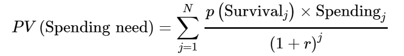
The numerator is the expected cash flow in year j, that is, the probability of surviving until that year times the spending in that year should the person survive.
This approach does not fully account for the risk inherent in capital markets. One way to adjust for this underestimation is to augment core capital with a safety reserve designed to incorporate flexibility into the estate plan.
Estimating Core Capital with Monte Carlo Analysis
Another approach to estimating core capital uses Monte Carlo analysis, a computer-based simulation technique that allows the analyst to forecast a range of possible outcomes based on, say, 10,000 simulated trials.
Rather than discounting future expenses, this approach estimates the size of a portfolio needed to generate sufficient withdrawals to meet expenses, which are assumed to increase with inflation. This approach more fully captures the risk inherent in capital markets than the mortality table approach described above.
One can incorporate recurring spending needs, irregular liquidity needs, taxes, inflation, and other factors into the analysis. In the context of calculating core capital, the wealth manager might estimate the amount of capital required to sustain a pattern of spending over a particular time horizon with, for example, a 95 percent level of confidence.
The safety reserve may also be added to accommodate flexibility in the first generation’s spending patterns. It need not be quite as large as that used in the mortality table method, however, because Monte Carlo analysis already captures the risk of producing a sequence of anomalously poor returns. In contrast to the mortality table method in which cash flows are discounted at the risk-free rate of return, the expected returns used in Monte Carlo analysis are derived from the market expectations of the assets comprising the portfolio.
Asset allocation affects the expected return and volatility of the portfolio, which in turn affects the sustainability of a given spending rate. Obviously, higher return improves sustainability and would require less core capital to generate the same level of spending. Volatility must also be considered, however, because it decreases the sustainability of a spending program for at least two reasons. First, even in the absence of a spending rule, volatility decreases future accumulations. This concept can be illustrated by noting that future accumulations per unit of currency are equal to the product of one plus the geometric average return, or:
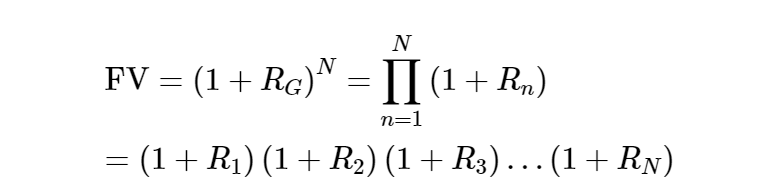
where RG is the geometric average return over period N. It is commonly referred to as the compounded return. The geometric average return is related to the arithmetic average return and its volatility in the following way:
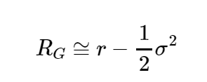
where r is the arithmetic average return and σ is the volatility of the arithmetic return. According to this, higher volatility decreases the geometric average return and hence future accumulations, which in turn decreases sustainability.
Another reason volatility decreases sustainability relates to the interaction of periodic withdrawals and return sequences. The above shows shows that future accumulations do not depend on the sequence of returns in the absence of periodic spending withdrawals. That is, the future value calculation is unchanged regardless of whether R1 and R2 (or any other two periodic returns) are reversed.
This independence disappears when withdrawals are introduced. Specifically, the sustainability of a portfolio is severely compromised when the initial returns are poor because a portion of the portfolio is being liquidated at relatively depressed values, making less capital available for compounding at potentially higher subsequent returns.
Monte Carlo analysis is commonly used in retirement planning. Depending on the sophistication of the model, the user can input the starting portfolio value and assumptions for:
- Distribution amounts, both recurring and irregular one-time distributions.
- Inflation rates.
- Asset class returns and correlations.
- Return distributions, either normal or non-normal.
- Tax rates.
- And any other relevant factors.
Hundreds or thousands of simulation runs can be generated and ranked with output displayed in various forms.
One common display would chart the value of the portfolio over time at some specified probability. Another display format is to show the probability of ruin (reaching a zero portfolio value) based on differing start dates for retirement (start of withdrawals) and distribution percentage. Delaying retirement or lowering the distribution percentage make it less likely the portfolio can be exhausted.