The foundation of statistical inference, which we use whenever we make decisions based on an analyst’s forecast of a company’s EPS or an economist’s forecast of the FED’s prime rate, is probability theory.
With probability theory, we attempt to calculate the likelihood of a specific outcome of a random variable occurring from a set of outcomes called events. If the set of events includes all possible outcomes for a variable, then we have an exhaustive set of events.
This gives us the two main properties of probability theory:
- The probability of any event (or subset of outcomes) occurring is between 0 and 1.
- The sum of the exhaustive set of events is 1.
There are three ways we make probability judgements. With empirical probability, we take the historical data to calculate the percent of the time an outcome occurs. We create subjective probabilities when we modify the results of empirical probabilities based on personal opinions and experience. This can be done if we believe underlying assumptions to be changing or if there is not enough data to create strong empirical probability. A combination of these two would lead to a priori probabilities, in which we used outcomes we know to make logical deductions about outcomes that aren’t certain. Of these two, only empirical and a priori probabilities are considered objective, in that they do not change from person to person.
When we determine the probability that a single even occurs on its own, we are calculating the unconditional probability of the event. If we are looking for the probability of an event, given another event occurring, this is a conditional probability. If an event occurring does effect the probability of another event occurring, then the two events are dependent. Otherwise they are independent.
- Unconditional Probability: P(A)
- Conditional Probability: P(A|B) = P(AB)/P(B) & P(B|A) = P(AB)/P(A)
- Independent Probabilities: P(A|B) = P(A) & P(B|A) = P(A)
The CFA has a little section on converting odds to probabilities and back.
- Odds for E = P(E)/(1-P(E)), which read as numerator (a) to denominator (b).
- Conversely, given odds (a) to (b), the probability is a/(a+b).
Probability Maths
From the properties above, we can derive certain equations that allow us to calculate joint probabilities, which is the combined probability of two more events happening, or P(AB)
The easiest type of to calculate is the joint probability independent events.
- P(AB) = P(A)P(B)
- P(ABC) = P(A)P(B)P(C)
- P(ABCD) = P(A)P(B)P(C)P(D) and so on.
In general, to find joint probabilities we use the multiplication rule for probability.
P(AB) = P(A|B)P(B) or P(B|A)P(A)
A related concept is the addition rule for probability, used for finding P(A or B)
- P(A or B) = P(A) + P(B) – P(AB)
The total probability rule allows us to determine the probably that an event (A) occurs based on the occurrence of a set of mutually exclusive events, (S) and its complement (Sc). The total probability rule allows us to solve for conditional probabilities when we do not know joint probabilities, or vice versa.
- P(A) = P(AS) + P(ASC) = P(A|S)P(S) + P(A|Sc)P(SC)
- P(A) = P(AS1) + P(AS2) + …. P(ASn) = P(A|S1)P(S1) + P(A|S2)P(S2) + … + P(A|Sn)P(Sn)
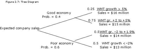
This equation is similar to weighted means, where the probability of the conditional event, P(A|S) is multiplied by the probability of all possible scenarios, P(S), giving us to total probability of the event, P(A).

In the diagram, we see the a visual of the total probability rule, where the total probability of expected sales (A) depends on the quality of the economy (S), which are conditional variables, P(A|S).
Expected Return and Variance of Portfolios
Moving onto to portfolio forecasting, we will build the total probability rule and apply it to find expected returns of a portfolio, which is the sum of the weighted return of each asset in the portfolio.
- Expected Return of an asset: ΣP(Ri) Ri
- Expected Return of an asset with conditional probability: E(R|S)P(S) + E(R|Sc)P(Sc) = ΣE(R|Si)P(Si)
- Expected Return of Portfolio: ΣwiE(Ri)
- Variance of a Probability: ΣP(xi)[(xi – E(X)]2
The variance of a portfolio is more complicated than a weighted average because we have to introduce the notion of covariance and correlation. The overall variance of a portfolio is dependent not just on each assets individual variance, but also the covariance between each asset.
- Variance of a Portfolio (2-asset): wa2σa2 + wb2σb2 + 2wawbCov(a,b)
For more than 2 assets, you must add the additional weighted covariance of each asset to one another. For instance, given 3 assets, the covariance values added to the sum of the weighted variances would be 2wawbCov(a,b), 2wawcCov(a,c), and 2wbwcCov(b,c).
- Covariance(a, b): σaσbρa,b
- Correlation(a,b): Cov(a,b)/σaσb
The main thing to know about correlation is that -1 is a perfect inverse linear relationship, 1 is perfect positive linear relationship and 0 is no linear relationship.
A similar relationship exists for covariance, where a negative covariance signifies that two assets tend to vary from there expected values in different directions, or have opposite skews. A positive correlation signifies that the stocks’ variances are skewed in the same direction, and a value of 0 means the two assets are unrelated. Finally, the covariance of an asset with itself is its variance.
Bayes’ Formula and Counting Equations
Another application of the total probability rule is Bayes’ Formula. This formula allows us to update our probabilities on an event given new information.
- Bayes’: P(Event|New Info) = [P(New Info|Event)/P(New Info)]P(Event)
In terms of counting methods to know, there is factorial counting, combinations, and permutations. Each has a function on the calculator so it is worth getting to know then. Factorial counting is used to calculate the realm of possibilities given n options and n spots, like the number of orders you can put 5 chairs. Combinations are used for calculating the possibilities given n options and r number of spots, where order does not matter. Permutations are used to compute the number of possibilities given n options, r spots, and where order does matter.
- Factorial: n!, where n is number of observations
- Combination: n!/((n-r)!r!), where n is number of observations, r is number of spots
- Permutation: n!/(n-r)!, where n is number of observations, r is number of spots
Finally there is an equation for general labeling, counting the number of ways n observations can be put into k number of spots.
- Multinomial Formula: n!/(n1!n2!…nk!)
