Statistics can refer to two different applications. Descriptive statistics take values in a data set and summarize them in order to make sense of the information in the set. Statistical inference uses probability theory and descriptive statistics to make estimates or forecasts about larger data sets given a smaller data set.
The data sets that are studied in statistics can be populations or samples. A data set on a population means that every member of a group is represented in the data. A sample data set on the other hand, only represents a portion of the population.
In descriptive statistics, we use parameters as the measures and summary tools to draw meaning from a data set. Common parameters are means, medians and variances. Because data sets covering populations are rare, we usually use sample parameters to make estimates about population parameters.
The most basic form of data measurement is scaling. By scaling, we categorize and sort the data. There are four types of scaling, nominal, ordinal, interval and ratio scales. Nominal scales are the weakest for of sorting, the data is categorized but not ranked. Ordinal scales categorize and rank data, but the rankings do not give information on relative differences. The exact difference between a higher and lower rank is not clear, nor is the difference between two members of the same rank. Interval scales rank and categorize, with the ranks determined on a scale with equal distance between each point in the scale. In other words, a data point can be assigned a numeric value, and all other points can be determined to be (x) values away from that point. Finally, ratio scales are intervals scales with a fixed zero point, allowing us to make comparisons between points in terms of ratios, such as (x) is three times as much as (y).
Frequency Distributions
The most basic way to summarize data is with a frequency distribution. We create frequency distributions by sorting in ascending order data, and then creating intervals within the range of data. By placing each point into the respective interval range, we can get feel to the dominant ranges in the set. The way to determine the size of each interval category depends on the number of categories we want. For instance, to sort data in quintiles we would divide the range of the data by 5. Each interval category would then span 1/5th of the range. Frequency distributions can be presented in graph form using histograms or line charts. The relative frequency of a range is the percent of observations in the interval category. The cumulative frequency of a range is the percent of observations in a given category and all those below.
To find a specific value (X) at a percentile (y), first calculate the location of the value:
- Ly = (n+1)(y/100).
The value (X) is then the value of the closest whole X + a percentage of the next X.
Central Tendency Measures
Measures of central tendency are parameters that describe where the center of data set lies.
- Arithmetic Mean: [Σ(Xi)]/n for (n) observations
This mean can refer to a population or sample. Means can be cross-sectional (at a specific time), or time-series (mean over time). Means are limited when a data set contains extreme values.
- Weighted Average Mean: ΣwiXi where the Σwi = 1.
- Geometric Mean: n√(x1x2x3…xn) for (n) observations. When using percentages, x1 = 1 + r1
The geometric mean allows us to better summarizes growth rates over time, or average change over time in time-series data.
- Harmonic mean: n/Σ(1/xi) for n observations.
Used for dollar cost averaging problems on the CFA, harmonic means are best used to average ratios. It is the smallest of the three Pythagorean means. Arithmetic means are the largest.
Modes and Medians are two other measures of central tendency. The median is the value occupying the middle position of the data set, and the mode it the value that occurs the most frequently.
Measures of Dispersion
Once we know the central tendency of a data set, the next most important parameter is how the actual values of the set differ from the mean. Like central tendency measures the[re are a variety of measures of dispersion. The most basic measure is Range, which is the difference between the min and max value.
- Mean Absolute Deviation: [Σ|Xi – X̄|]/n, where (n) is the number of observations
- Population Variance: [Σ(Xi – µ)2]/n, where (n) is the number of observations, also notated as σ2
- Sample Variance: [Σ(Xi – x̄)2]/(n – 1), where (n) is the number of observations
- Standard Deviation: √(variance), also notated as (σ).
For semi-variances, we calculate the data mean but only find the sum squared average deviations that are below or above the target value. In the variance equations above, we would add the condition:
- Population semi-variance: [Σ(Xi – µ)2]/n, where (n) is the number of observations, For all Xi < or > Xt.
- Chebychev’s Inequality is a relationship equation that determines that the percent of observations that fall within k standard deviations of the mean is at least 1-1/k2 for all k > 1.
By dividing the standard deviation of the set with the sample mean, we can a relative measure of dispersion from the mean which allows us to compare dispersion between data sets which may differ in some way, like scale. This value is the Coefficient of Variation.
- Coefficient of Variation: std/X̄
A concept related to the coefficient of variation is the Sharpe Ratio, which is based on the inverse of the coefficient.
- Sharpe Ratio: (r̄p – rf)/σ
In the above, we are measure excess return per unit of standard deviation above the risk free rate, but we could use any target rate for rf. The higher the ratio, the better the performance.
Third and Fourth Degree descriptors
In terms of mathematics, mean and variance are based on first and second degree derivatives. They can be related concepts of slopes and change in slopes on a curve. Two more statistical parameters the CFA expects us to know are Skewness and Kurtosis. In this allegory, skewness and kurtosis are third and fourth degree derivatives in differential calculus.
Skewness measures the degree that a distribution is left or right leaning. A positive skew of the variances means that there are more frequent, or larger positive variances than there are negative variances. A symmetrical distribution has a skewness of 0. What is confusing about skewness is the graphical representations.
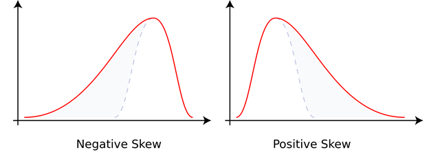
Intuitively, I would imagine that a positive skew would be a larger peak on the right hand side of the graph, not on the left hand side as this shows. However, skewness in these graphs is not based on area under the curve but on the length of the tail. The positive skew has the longer tail on the right hand side.
- Skewness: [n/((n-1)(n-2))][Σ(xi – x̄)3/σ3] where normal distributions have skew of 0
Kurtosis is the measure of the concentration of observations around the mean. The more peaked a distribution appears, the greater the concentration of observations lies around the mean. This is called a leptokurtic distribution, meaning slender. The opposite would be a platykurtic distribution, meaning broad. A mesokurtic distribution would lie in the middle as the normal distribution.
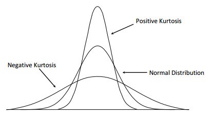
- Kurtosis: (1/n)[ Σ(xi – x̄)4/σ4] – 3, for large number of observations, where 0 is normal distribution