
Estimating a single variance that is believed to be constant is straightforward: The familiar sample variance is unbiased and its precision can be enhanced by using higher-frequency data. The analyst’s task becomes more complicated if the variance is not believed to be constant or the analyst needs to forecast a variance–covariance (VCV) matrix.
The VCV Matrix
Estimating a constant VCV matrix can most easily be done from deriving variances and covariances from sample statistics.
The main advantage of using multifactor models for VCV matrices is that it significantly reduces the number of required observations.
The return of the ith asset in a multifactor model can be calculated as:
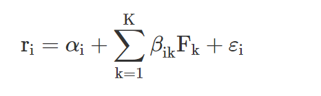
where K represents the number of common factors, αi is the intercept, βik is the ith asset’s sensitivity to the kth factor, Fk is the kth factor return, and εi is a factor term unique to asset i with a zero mean.
The variance of the ith asset can be derived as:
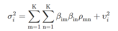
where ρmn is the covariance between the mth and nth factors, and vi2 is the variance of the εi unique factor.
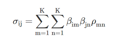
The last step is to look at the covariance between the ith and jth asset:
Assuming these factors are not redundant and do not have zero terms will help us ensure that the matrix outcomes are not meaningless and that portfolios do not incorrectly appear riskless.
Despite their significant advantages, factor-based VCV matrices have several shortcomings:
- The matrix is biased: Matrix inputs need to be estimated and will be misspecified. As a result, the matrix will be biased, meaning it will not be a predictor of the true returns, not even on average.
- The matrix is inconsistent: As the sample size increases in the factor-based VCV matrix, the model does not converge to the true matrix. In contrast, the sample VCV matrix will be both consistent and unbiased.
Shrinkage Estimates
Combining information in the sample VCV matrix with a target matrix (e.g., the factor-based VCV matrix) will result in more precise data and reduced estimation error. The shrinkage estimate is a weighted average estimate of the sample and target (e.g., factor-based) matrix, with the same weights used for all elements of the matrix, including the variance and covariance factors. The resulting figures will be more efficient because they will have smaller error terms.
Smoothed Returns to Estimate Volatility
Smoothing of data leads to underestimating risk and overstating returns and diversification benefits. Not adjusting for smoothing tends to lead to distorted portfolio analysis and suboptimal asset allocation decisions. As a result, it is important that analysts adjust the data for the impact of smoothing.
ARCH Models
Asset returns generally show periods of high and low volatilities, leading to volatility clustering. These volatilities can be addressed through autoregressive conditional heteroskedasticity (ARCH) models.
The simplest ARCH formula can be written as:
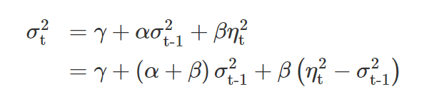
where α, β, and γ are nonnegative parameters and (α + β) < 1, and ηt is a random variable indicating the unexpected return component.
Higher α + β terms indicate higher emphasis on past information, leading to volatility clustering.