Module 9.2 LOS 9.h (And General Times Series: Instability of Coeffiecients in Time Series Models

Time Series

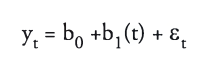
We can use regression models for time series as well. The two basic time series graphs are the linear time series:

and log-linear time series models:

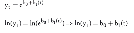
These model specifications are not much different from normal regression specifications.

However, time series regressions are especially prone to serial correlation, misspecification and heteroskedasticity, so more complicated regression methods are presented in the material that allow us to obtain better outputs for time series regressions.

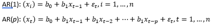
Autoregressive Models

Autoregressive models allow us to regress a dependent variable against one or more lagged values of itself.

Autoregressive models can also exhibit serial correlation, however the DW statistic is not applicable in this case. Instead we use a t-test to determine if the correlations between the residuals at any lag are significant. If serial correlation is present, we can add an additional lagged variable to correct the model specification.

A requirement of AR models is that the time series must be covariance stationary. Covariance stationarity occurs if the following three conditions are satisfied:

• The expected value of the time series is constant over time (constant finite mean)
• The time series volatility around its mean does not change over time (constant finite variance)
• The covariance of the time series with leading or lagged values is itself constant.

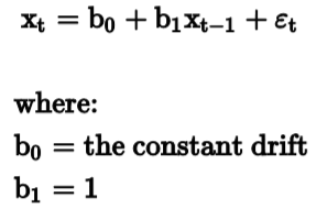
The Dickey-Fuller test is necessary to determine whether an AR model is covariance stationary. The D-F test is a test for unit root, in other words, if B₁ – 1 = 0. If B₁ – 1 = 0 is not significantly different from zero, then it can be said that B₁ = 1, and the series has unit root. In this case it is not covariance stationary and there is no mean reverting level:

We can use first differencing to eliminate unit root.

Random Walk Processes

Random walk processes are AR(1) models which are non-covariance stationary –  or in other words, have a b₁ value not significantly different than one.

These models are said to exhibit unit root. In this case, the best predictor of x_t is simply x_t-1: and

1. The expected value of each error term is zero
2. The variance of the error terms is constant
3. There is no serial correlation in the error terms

A subset of random walk AR(1) models are random walks with a drift, which has the same properties except that the b₀ (intercept) value does not equal zero.

Issues with AR(1) time series models

Seasonality refers to a cyclical pattern displayed in the regression data. AR models must be adjusted by adding a lagged term to correctly specify the regression.

Autoregressive conditional heteroskedasticity exists is the variance of residuals in one period is dependent on the variance of residuals in the previous period. This leads to invalid standard errors of regression coefficients and invalid coeffecients.

We test for ARCH using ARCH(1) models,

 

 

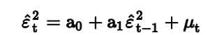
Where if a₀ is significantly different from 0, the series has ARCH. We correct using methods such as generalized least squares.

Regressions with Two Time Series

In certain cases, we run a regression with two time series. In this situation, both time series can exhibit unit root and we must test for this condition to determine the validity of the regression. The following options are possible:

1. One unit root – linear regression not valid
2. Two unit roots – test variables for cointegration
3. No unit roots – linear regression valid

Cointegration means that the two variables are linked and allows for a valid regression even if unit root is present. We test for cointegration using the Dickey-Fuller Engle and Granger test.

Table of Contents