
Regression Model Assumptions
Linear Regression Models operate under the following assumptions:
- A linear relationship exists between dependent and independent variables
- The independent variable is uncorrelated with the residual term
- The expected value of the residual term is zero
- There is a constant variance with of the residual term
- The residual term is independently distributed; that is, the residual term for one observation is nor correlated with that of another observation
- The residual term is normally distributed
Not all models meet the necessary assumptions, and beyond that there are various challenges that are involved in linear regression models. The following are some ways in which models can give invalid outputs. These errors can occur in both simple linear regression as well as multivariable regression models.
Model Misspecification
First, we look at model misspecification. Model specification is the selection of independent variables which we believe to be inputs to our dependent variable. Misspecification occurs when our inputs or equation is made in a way that will biased or inconsistent, this reducing our confidence in the value of our outputs.
Some ways models can be misspecified include:
- Omitting variables which should be in model, whether as stated necessary inputs or logical inputs.
- Ignoring necessary variable transformations when data need to be corrected in order to show a linear relationship between independent and dependent variables
- Incorrectly pooling data, most commonly using data from in different time periods, or data from one long time period in which different relationships occur
- Using lagged dependent variables as independent variables – for instance trying to find a relationship between the same variable in times t and t-1.
- Forecasting the past, when the t of dependent and independent variable don’t match, creating a situation where we are using for example, end of month values to forecast average month values.
- Measuring independent variables with error – occurs when we incorrectly us proxy variables
The next step of model validating a model is to check for three common Regression problems.
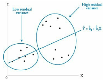
Heteroskedasticity
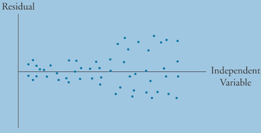
Heteroskedasticity occurs when the variance of the residuals is not constant across all observations. We are concerned with conditional heteroskedasticity, which leads to unreliable standard error estimates. Because coefficient estimates are not impacted, t-statics will be too large.
Conditional heteroskedasticity means that the residual variance is related to the level of the independent variable.
We can detect heteroskedasticity with the Breusch- Pagan Chi-squared test:

- Where R2 is the sum of the square residuals, different from the regression R2.
We correct for heteroskedasticity using robust standard errors, or White-corrected standard errors.
Serial Correlation
Serial Correlation or autocorrelation is a common problem that arises in regression tests when residual errors are correlated with one another. Like heteroskedasticity, this breaks the requirement for residual error terms to be random and independent, and just like heteroskedasticity, this leads to type I errors. In other words our t-values will be too large and we will reject too many null hypothesis.
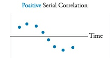
There are two types of serial correlation, positive and negative. Positive serial correlation can be describer like a residual error snowball, where each residual error effects the next period error.
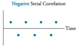
Negative serial correlation can be described as when a positive residual increases the probability of a negative residual in the next period, and vice versa.
Serial collinearity can be detected with the Durbin-Watson statistic. This is usually denoted as DW. Also note that for large samples, the adjusted DW = 2(1-r).
Where r is the correlation coefficient between the residuals
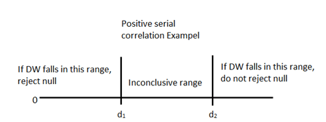
A DW value of 2 indicates homoskedasticity and no serial correlation. A DW of less than 2 indicates positive serial correlation and a DW greater than 2 indicates negative serial correlation. We use significance testing to determine how much of a difference is required in order for serial correlation to be present.
Null Hypothesis: There is no positive/negative serial correlation
We can remedy serial correlation error by adjusting the coefficient of standard errors with the Hansen method, or respecify our model into a time series. Note that the Hansen method also corrects for heteroskedasticity, but the White method is better when there is only heteroskedasticity error.
Multicollinearity
Multicollinearity occurs when two or more independent variables in a model are highly correlated with one another. Since standard error of the estimate and of the coefficient will be distorted, we will experience unreliable t-statistics. This leads to a Type II error where we have a greater probability of concluding that variables are not statistically significant.
The main symptom of multicollinearity from the material is when t-tests indicate that the individual coefficients of a the regression are not significantly different from 0, but the F-test is significant and the R2 is high.
Correcting multicollinearity requires identifying the correlated variables, using a stepwise regression for instance, and removing the offenders.