
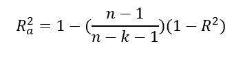
The R2 (adjusted vs unadjusted)
The R2 value is the also called the coefficient of determination. It is a numerical representation of how well the values tested fit the regression equation. With an R2 value of 0.40, for example, you could say that 40% of the movement in the independent variable explains movement in the dependent variable.
For multi-variable regressions, there is an also the adjusted R2 value, which adjusts for the number of independent variables and polynomials you are considering in the regression (see end of post for eqn). This is done to solve two issues with an unadjusted R2 value:
- Adding additional inputs will always increase the R2, regardless of model
- As the number of predictors and polynomials increase, noise increases in the model
ANOVA
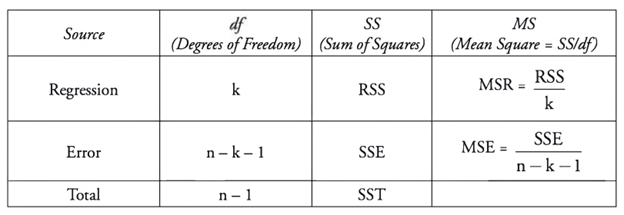
ANOVA is short for analysis of variance. The key concept is the sum of squared deviations. The goal is to dig into the differences between observed values, the observed mean and our regression line.
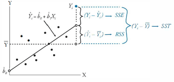
The Total Sum of Squares, or SST is the sum of the deviations of each observed value from the population mean. For example, given observed values of 1, 2, 3 we have a population mean, or simple average of 2. SST is also two in this case, as SST = (2-1) + (2-2) + (3-2) = 2.
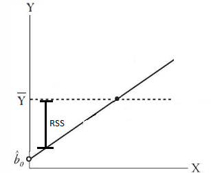
The regression sum squared, or RSS is the difference between each point of the regression line of our model and the population mean. In the example above, because we have a linear equation that fits the observed points perfectly (y = x), the RSS = SST. This is called the explained variation, because it is variation from the population mean that our model (line) explains.
Moving onto the residual sum of square errors, or SSE, we have the sum of the differences between the observed values and the regression line. Consider if the observed values where 1.2, 2, 2.8, our linear regression line would likely still be y = x. This means the population mean would still be 2 and the RSS would still be two as well, since our model is assumed to not have changed. However, now we cannot say that RSS = SST, because the observed values are no longer perfectly on the regression. There is an additional variation between the observed value and the linear regression line. This is the SSE, and SST = RSS + SSE. SSE is also known as unexplained variation, as it lies outside of what is predicted by our regression line. In an optimized regression, the lower the SSE, the better the regression fits the data.
Calculating R2 and SEE
From the ANOVA components, we can derive that R2 = RSS/SST. We see this means that the R2 value indicates how much of the variance between the observed value and the population mean is explained by our regression line.

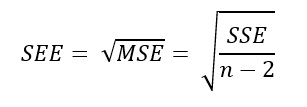
The standard error of estimate (SEE) measures the degree that estimated Y-values vary from actual Y-values. It could be said to be a measure of how well our the regression line fits our observations.
There is also an adjusted R2 value, which adjusts the value for the number of variables being tested (Multiple regression):
The F-statistic
Using the F-test we can determine how well a group of independent variables explain the variation in the dependent variables. When there are numerous independent variables, the F-test indicates whether at least one of the independent variables are significant.
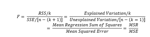
The F-test tests a null hypothesis that all the coefficients equal zero. If we reject the null hypothesis because the F-statistic is greater than the critical value, this means that at least one of the coefficients is significantly different from zero, and therefore significantly contributes to the explanation of the dependent variable.
We can also use the p-value as a test of our test statistics. In this case, the p-value is a probability that indicates the likelihood that our test statistic would be generated when the null hypothesis is true.
Let’s say we reject the null hypothesis based on an F-test value of 230, where the critical value is 160. If we have a P-value of .001, that means that there is a 0.001% chance that we would generate a F-test value of 230 under circumstances where our regression coefficients did equal zero. In other words, there is a 0.001% chance that we have incorrectly rejected the null hypothesis. However, if the p-value where .85, this would indicate an 85% chance that the value 230 could be generated when our coefficients equal zero, which would lead us to question our model’s validity.
In short, a low p-value for a test statistic agrees with rejecting a null hypothesis, while a higher p-value favors the null hypothesis.