
Monte Carlo Simulation
Monte Carlo simulation complements MVO by addressing the limitations of MVO as a single-period framework.
In the case in which the investor’s risk tolerance is either unknown or in need of further validation, Monte Carlo simulation can help paint a realistic picture of potential future outcomes, including the likelihood of meeting various goals, the distribution of the portfolio’s expected value through time, and potential maximum drawdowns.
Benefits of Monte Carlo Simulation for Retirement Planning
- It can incorporate path dependency issues such as how past distributions during periods of depressed portfolio value may lead the portfolio to be depleted sooner.
- It focuses manager and client attention on the more relevant issue of longevity risk instead of on the short-term issue of volatility of assets or of surplus.
- It is superior for multiperiod analysis because it treats modeling as a stochastic process, incorporating both starting portfolio value as well as additions and withdrawals during each period.
- It can display probabilistic projected value of the portfolio at future points in time, facilitating client discussion of when to retire and how much to save.
- It can better incorporate other factors such as taxes.
Criticisms of Mean–Variance Optimization
- The outputs (asset allocations) are highly sensitive to small changes in the inputs.
- The asset allocations tend to be highly concentrated in a subset of the available asset classes.
- Many investors are concerned about more than the mean and variance of returns, the focus of MVO.
- Although the asset allocations may appear diversified across assets, the sources of risk may not be diversified.
- Most portfolios exist to pay for a liability or consumption series, and MVO allocations are not directly connected to what influences the value of the liability or the consumption series.
- MVO is a single-period framework that does not take account of trading/rebalancing costs and taxes.
Addressing the Criticisms of Mean–Variance Optimization
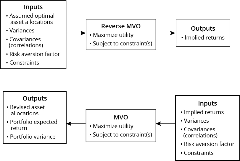
Reverse optimization is a powerful tool that helps explain the implied returns associated with any portfolio. It can be used to estimate expected returns for use in a forward-looking optimization. Reverse optimization takes as its inputs a set of asset allocation weights that are assumed to be optimal and, with the additional inputs of covariances and the risk aversion coefficient, solves for expected returns. These reverse-optimized returns are sometimes referred to as implied or imputed returns.
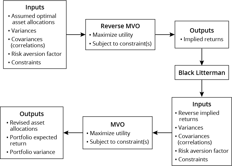
The Black-Litterman model is an extension of reverse optimization in which the implied returns from a reverse optimization are subsequently adjusted to reflect the investor’s unique views of future returns.
Adding constraints beyond the budget and nonnegativity constraint can be used to address the GIGO and highly concentrated allocation issues.
Typical examples of additional constraints include:
- Specifying a fixed allocation to one or more assets, often human capital or other nontradable assets.
- Setting an asset allocation range for an asset class
- Setting an upper limit on the asset allocation to an asset class to address liquidity issues
- Specifying a relative allocation between two or more classes
- In a liability-relative setting, including a constraint to require an allocation to assets that hedge the liability.
Resampling can also be used to address the GIGO and highly concentrated issues. Resampling starts with the basic MVO using the best estimates of expected returns, sigma, and correlations to generate the efficient frontier and associated asset allocations for each point on the frontier. Then Monte Carlo simulation is used to generate thousands of random variations for the inputs around the initial estimates, resulting in efficient frontier and associated asset allocations for each point on the frontier. The resampled efficient frontier is an average of all the simulated efficient frontiers, and the asset allocation for any single point on the resampled efficient frontier is an average of the possible portfolios for that point on the frontier.
The third critique of MVO, that it ignores skewness and kurtosis in asset returns, can be addressed by various extensions of MVO. You could directly incorporate skewness, kurtosis, or both into the utility function and use an asymmetric definition of risk, such as conditional value-at-risk (VAR), instead of variance.
| Key Non-Normal Frameworks | Research/Recommended Reading |
|---|---|
| Mean–semivariance optimization | Markowitz (1959) |
| Mean–conditional value-at-risk optimization | Goldberg, Hayes, and Mahmoud (2013) Rockafellar and Uryasev (2000) Xiong and Idzorek (2011) |
| Mean–variance-skewness optimization | Briec, Kerstens, and Jokung (2007) Harvey, Liechty, Liechty, and Müller (2010) |
| Mean–variance-skewness-kurtosis optimization | Athayde and Flôres (2003) Beardsley, Field, and Xiao (2012) |