
Mean-variance optimization (MVO) is the most common approach to asset allocation. It assumes investors are risk averse, so they prefer more return for the same level of risk.
Markowitz recognized that whenever the returns of two assets are not perfectly correlated, the assets can be combined to form a portfolio whose risk (as measured by standard deviation or variance) is less than the weighted-average risk of the assets themselves.
An additional and equally important observation is that as one adds assets to the portfolio, one should focus not on the individual risk characteristics of the additional assets but rather on those assets’ effect on the risk characteristics of the entire portfolio.
Mean–variance optimization requires three sets of inputs: returns, risks (standard deviations), and pair-wise correlations for the assets in the opportunity set. The objective function is often expressed as follows:
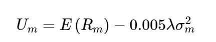
where
Um = the investor’s utility for asset mix (allocation) m
Rm = the return for asset mix m
λ = the investor’s risk aversion coefficient
σ2m = the expected variance of return for asset mix m
Given an opportunity set of investable assets, their expected returns and variances, as well as the pairwise correlations between them, MVO identifies the portfolio allocations that maximize return for every level of risk.
If the MVO analysis includes all investable risky assets, the result is the “efficient frontier” as shown in Mean-Variance Efficient Frontier.

The slope of the efficient frontier is greatest at the far left of the efficient frontier, at the point representing the global minimum variance portfolio. Slope represents the rate at which expected return increases per increase in risk.
Maximization problems in general usually also have constraints. These are restrictions on the variables in the objective function. In MVO, the constraints typically involve the portfolio weights, but they can also reflect restrictions on portfolio expected return, variance, or both.
The most common constraint in MVO is called the budget constraint or the unity constraint, which means the asset weights must add up to 100%.
The next most common constraint used in MVO is the nonnegativity constraint, which means all weights in the portfolio are positive and between 0% and 100%.
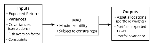
A graphical depiction of MVO is shown in MVO Process.
Criticisms of MVO
- GIGO: The quality of the output from the MVO is highly sensitive to the quality of the inputs (i.e., expected returns, variances, and correlations).
- Concentrated asset class allocations: MVO often identifies efficient portfolios that are highly concentrated in a subset of asset classes, with zero allocation to others.
- Skewness and kurtosis: MVO analysis, by definition, only looks at the first two moments of the return distribution: expected return and variance; it does not take into account skewness or kurtosis.
- Risk diversification: MVO identifies an asset allocation diversified across asset classes but not necessarily the sources of risk.
- Ignores liabilities: MVO also does not account for the fact that investors create portfolios as a source of cash to pay for something in the future.
- Single-period framework: MVO is a single-period framework that does not take into account interim cash flows or the serial correlation of asset returns from one time period to the next.